Guide
Introduction
snipar (single nucleotide imputation of parents) is a Python package for inferring identity-by-descent (IBD) segments shared between siblings, imputing missing parental genotypes, and for performing family based genome-wide association and polygenic score analyses. snipar provides a script for estimating the different effects estimated by family-GWAS. snipar also contains a module for simulating traits affected by assortative mating with and without indirect genetic effects.
snipar can perform family-GWAS and family-PGS analyses with and without imputed parental genotypes.
snipar can impute missing parental genotypes for any samples who have at least one genotyped full-sibling and/or parent.
The imputation method and the family-based GWAS and polygenic score models are described in Young et al. 2022.
A method for adjusting family-PGS analyses for assortative mating is described in Young et al. 2023.
Additional family-GWAS estimators that maximize power by inclusion of samples without genotyped first-degree relatives and for samples with strong structure and/or admixutre (the robust estimator) are described in Guan et al. 2025. This paper also describes the linear mixed model implemented in snipar for family-GWAS and PGS analyses: this models correlations between siblings and between other relatives using a sparse genetic relationship matrix, GRM.
Installation
snipar currently supports Python 3.7-3.9 on Linux, Windows, and Mac OSX. We recommend installing using pip in an Anaconda environment as the most reliable way to install snipar and its dependencies.
Installing Using pip
The easiest way to install is using pip:
pip install snipar
Sometimes this may not work because the pip in the system is outdated. You can upgrade your pip using:
pip install –upgrade pip
You may encounter problems with the installation due to Python version incompatability or package conflicts with your existing Python environment. To overcome this, you can try installing in a virtual environment. In a bash shell, this could be done by using the following commands in your directory of choice:
python -m venv path-to-where-you-want-the-virtual-environment-to-be
You can activate and use the environment using
source path-to-where-you-want-the-virtual-environment-to-be/bin/activate
snipar can also be installed within a conda environment using pip.
Installing From Source
To install from source, clone the git repository (https://github.com/AlexTISYoung/snipar), and in the directory containing the snipar source code, at the shell type:
pip install .
Python version incompatibility
snipar does not currently support Python 3.10 or higher due to version incompatibilities of dependencies. To overcome this, create a Python3.9 environment using conda and install using pip in the conda environment:
conda create -n myenv python=3.9
conda activate myenv
pip install snipar
Running tests
To check that the code is working properly and that the C modules have been compiled, you can run the tests using this command:
python -m unittest snipar.tests
Workflow
A typical snipar workflow for performing family-GWAS using imputed parental genotypes (see flowchart below) is:
Inferring identity-by-descent (IBD) segments shared between siblings (ibd.py)
Imputing missing parental genotypes (impute.py)
Estimating direct genetic effects and non-transmitted coefficients (NTCs) of genome-wide SNPs (gwas.py)
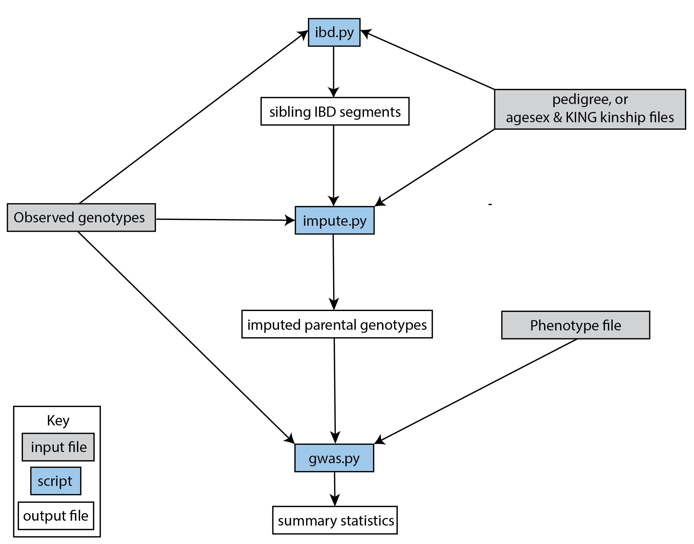
Illustration of a typical workflow for performing family-based GWAS
A snipar workflow requires input files in certain formats. See input files. Output files are documented here.
The tutorial allows you to work through an example workflow before trying real data.
Note that family-GWAS can be performed without imputed parental genotypes. See the simulation exercise.
Inputting multiple chromosomes
We recommend splitting up observed genotype files by chromosome since certain scripts in snipar cannot handle observed genotype files with SNPs from multiple chromosomes.
To run scripts for all chromosomes simultaneously (recommended), the @ character can be used as a numerical wildcard. For example, if you had observed genotype files chr_1.bed, chr_2.bed, …, chr_22.bed, then you could specify these as inputs to the command line scripts as “–bed chr_@”. If you only want to analyse a subset of the chromosomes, you can use the “–chr_range” argument; for example, ‘–bed chr_@ –chr_range 1-9’ would specify analysing observed genotype files chr_1.bed, chr_2.bed, …, chr_9.bed.
This will result in output files that are also split by chromosome. The names of the output files can also be specified using the numerical wildcard character, @, e.g. ‘–out /path/to/output/dir/chr_@’.
Inferring identity-by-descent segments
If your sample contains full-sibling pairs (without both parents genotyped), it is necessary to first infer the identity-by-descent (IBD) segments shared between the siblings before imputing the missing parental genotypes. If your sample does not contain any full-sibling pairs, but has genotyped parent-offspring pairs (i.e. one parent’s genotype is missing), imputation can proceed without inferring IBD.
snipar contains a Hidden Markov Model (HMM) algorithm for inferring IBD shared between siblings, which can be accessed through the command line script ibd.py.
The ibd.py script requires the observed genotypes of the siblings and information on the sibling and parent-offspring relations in the genotyped sample.
To infer IBD, one can use a smaller set of genetic variants than one intends to use in downstream analyses (imputation, gwas, etc.). For example, one could use the variants on a genotyping array to infer IBD segments, and these IBD segments could be used to impute missing parental genotypes for a larger set of variants imputed from a reference panel. This can be useful since the accuracy of IBD inference plateaus as the density of variants increases, so inputting millions of variants imputed from a reference panel to ibd.py will result in a long computation time for little gain in accuracy over using variants from a genotyping array.
The information on the relations present in the genotyped sample can be provided through a pedigree file or through the output of KING relationship inference (as output using the –related –degree 1 options: see https://www.kingrelatedness.com/manual.shtml#RELATED) along with a file giving the age and sex information on the genotyped sample. (The age and sex information along with the parent-offspring and sibling relations inferred by KING are used to construct a pedigree if a pedigree is not provided.)
The algorithm requires a genetic map to compute the probabilities of transitioning between different IBD states. If the genetic map positions (in cM) are provided in the .bim file (if using .bed formatted genotypes), the script will use these. Alternatively, the –map argument allows the user to specify a genetic map in the same format as used by SHAPEIT (https://mathgen.stats.ox.ac.uk/genetics_software/shapeit/shapeit.html#formats). If no genetic map is provided, then the deCODE sex-averaged map on GRCh38 coordinates (Halldorsson, Bjarni V., et al. “Characterizing mutagenic effects of recombination through a sequence-level genetic map.” Science 363.6425 (2019).), which is distributed as part of snipar, will be used.
The HMM employs a genotyping error model that requires a genotyping error probability parameter. By default, the algorithm will estimate the per-SNP genotyping error probability from Mendelian errors observed in parent-offspring pairs. However, if your data does not contain any genotyped parent-offspring pairs, then you will need to supply a genotyping error probability. If you have no external information on the genotyping error rate in your data, using a value of 1e-4 has worked well when applied to typical genotyping array data.
The HMM will output the IBD segments to a gzipped text file with suffix ibd.segments.gz. As part of the algorithm, LD scores are calculated for each SNP. These can also be output in LDSC format using the –ld_out option.
Imputing missing parental genotypes
impute.py is responsible for imputing the missing parental genotypes. This is done for individuals with at least one sibling and/or parent genotyped but without both parents genotyped.
You should provide the script with identity-by-descent (IBD) segments shared between the siblings if there are genotyped sibling pairs in the sample. Although we strongly recommend using IBD segments inferred by ibd.py, we also support IBD segments in the format that KING outputs (see https://www.kingrelatedness.com/manual.shtml#IBDSEG). If IBD segments in KING format are used, it is necessary to add the –ibd_is_king flag.
The script needs information about family structure of the sample. You can either supply it with a pedigree file or let it build the pedigree from kinship and agesex files.
If you are imputing for a chromosome with a large number of SNPs, you may encounter memory issues. If this is the case, you can use the –chunks argument to perform the imputation in chunks. When the script is run with ‘-chunks x’, it will split the imputation into ‘x’ batches. Alternatively, you can do the imputation for only on a subset of SNPS by using -start and -end options.
For each chromosome, imputed parental genotypes and other information about the imputation will be written to a file in HDF5 format. The contents of the HDF5 output, which a typical user does not need to interact with directly, are documented here.
The expected proportion of variants that have been imputed from a sibling pair in IBD0 (i.e. the parental alleles are fully observed) can be computed from the pedigree. At the end of the imputation, the script will output the expected IBD0 proportion and the observed IBD0 proportion. If there have been issues with the imputation (such as failure to match IBD segments to observed genotypes), this will often should up as a large discrepancy between expected and observed IBD0 proportions.
Family-based genome-wide association analysis
Family-based GWAS is performed by the gwas.py script. This script estimates direct genetic effects and (when using designs with observed/imputed parental genotypes) and non-transmitted coefficients of the input variants — the population effects, as estimated by standard GWAS. The phenotype specified in the phenotype file. (If multiple phenotypes are present in the phenotype file, the phenotype to analyse can be specified by its column name using the ‘–phen’ argument and by its column index using the ‘–phen_index’ argument, where ‘–phen_index 1’ corresponds to the first phenotype.)
If imputed parental genotypes are not provided, the default behaviour of the gwas.py is to perform a meta-analysis of samples with genotyped siblings but without both parents genotyped — using the sib-difference estimator — and samples with both parents genotyped — using the trio design. This should achieve something close to optimal power for family-GWAS without imputed parental genotypes. However, improved power can be achieved by using designs that take advantage of imputed parental genotypes.
When imputed parental genotypes are provided, the default behaviour of the gwas.py the script performs a regression of an individual’s phenotype onto their genotype, their (imputed/observed) father’s genotype, and their (imputed/observed) mother’s genotype. This estimates the direct genetic effect of the variant, and the paternal and maternal non-transmitted coefficients (NTCs). See Young et al. 2022 for more details.
If no parental genotypes are observed, then the imputed maternal & paternal genotypes become perfectly correlated. In this case, to overcome collinearity, gwas.py will perform a regression of an individual’s phenotype onto their genotype, and the imputed sum of their parents’ genotypes. This will estimate the direct effect of the SNP, and the average NTC. One can include the ‘–parsum’ argument to manually enable this option.
If one wishes to model indirect genetic effects from siblings, one can use the ‘–fit_sib’ option to add the genotype(s) of the individual’s sibling(s) to the regression.
To improve power when imputed and/or observed parental genotypes are available, the ‘–impute_unrel’ argument can be used to include samples without genotyped parents/siblings through linear imputation of parental genotypes. This can increase the effective sample size by up to 50% when very large samples without genotyped relatives are available. See the discussion of the unified estimator in Guan et al. 2025 for more details. If applied to the full sample for which standard GWAS would be applied, this method will give estimates of population effects of equivalent power to standard GWAS along with direct genetic effect estimates.
Methods with imputed parental genotypes can be susceptible to population stratification when samples are strongly structured (Fst > 0.01) or when parents are admixed between similarly differentiated groups. To maximize power in these cases, one can use the ‘–robust’ argument to use the robust estimator. This requires parental genotypes imputed from phased data to work, although the imputed parental genotypes are not directly used in regression design: the imputation procedure is used to work out parent-of-origin of alleles to enable optimal use of samples with one parent genotyped. See the tutorial for an example of how to use this option. The default behaviour of the gwas.py script is also appropriate for strongly structured samples, but will generally have reduced power compared to the robust estimator. See Guan et al. 2025 for more details
By defualt the gwas.py script estimates a variance component model that models the phenotypic correlation between siblings after accounting for the covariates. Modelling correlations between siblings is important to ensure statistically efficient estimates of direct genetic effects are obtained from samples with siblings. If a GRM is provided, an additional variance component will be added that models the correlation between individuals with genetic relatedness passing a chosen threshold specified by the ‘–sparse_thresh’ argument (default is 0.05).
Note that if no imputed parental genotypes are input, a pedigree file is required. (A pedigree input is not needed when inputting imputed parental genotypes.)
The script processes chromosome files sequentially, and allows parellel processing of each chromosome if ‘–cpus [NUM_CPUS]’ is used. One can also provide the number of threads used by NumPy and Numba for each CPUs by providing ‘–threads [NUM_THREADS]’. We recommend increasing ‘–cpus’ rather than ‘–threads’ for most users.
The script outputs summary statistics in both gzipped text format and HDF5 format.
Family-based polygenic score analyses
As in previous work (e.g. Kong et al. 2018: https://www.science.org/doi/abs/10.1126/science.aan6877), parental polygenic scores can be used as ‘controls’ to estimate the within-family association between phenotype and PGS, which only reflects direct genetic effects. In Young et al. 2022, we showed how this can be done using parental PGSs computed from imputed parental genotypes. snipar provides a script, pgs.py, that can be used for computing and analysing PGSs using observed/imputed parental genotypes.
The pgs.py script takes similar inputs to the gwas.py script. The main addition is that in order to compute a PGS, a weights file must be provided.
By default, if no phenotype file is provided, the pgs.py script will compute the PGS values of all the genotyped individuals for whom observed or imputed parental genotypes are available. The script will output a PGS file, including the imputed/observed PGS values for each individual’s parents, facilitating family-PGS analyses.
If the ‘–fit_sib’ argument is provided, the PGS file will include a column corresponding to the average PGS value of the individual’s sibling(s).
To estimate the direct and population effects as well as the non-transmitted coefficients (NTCs) of the PGS on a phenotype, input a phenotype file to pgs.py. One can first compute the PGS and write it to file, and then use this as input to pgs.py along with a phenotype file.
The direct effect and NTCs of the PGS are estimated as fixed effects in a linear mixed model that includes a random effect that models (residual) phenotypic correlations between siblings. By providing a GRM, correlations between other relatives can also be modelled. The population effect is estimated from a separate regression model that includes only the proband PGS (no control for parental PGS). The estimates and their standard errors are output to file along with a separate file giving the sampling variance-covariance matrix of the direct effect and NTCs.
See the simulation exercise for an example of how to use the pgs.py script. This also shows how the PGS script can be used to adjust the results of family-PGS analysis for the impact of assortative mating.
Estimating correlations between effects
As part of Tan et al. 2024, we estimated the genome-wide correlations between direct genetic effects and population effects and between direct genetic effects and average non-transmitted coefficients (NTCs). The correlation between direct genetic effects and population effects is a measure of how different direct genetic effects and effects estimated by standard GWAS (population effects) are.
We provide a script, correlate.py, that estimates these correlations. It takes as input the summary statistics files output by gwas.py and LD-scores for the SNPs (as output by ibd.py or by LDSC). It applies a method-of-moments based estimator that accouts for the known sampling variance-covariance of the effect estimates, and for the correlations between effect estimates of nearby SNPs due to LD.
Note that this is different to genetic correlation as estimated by LDSC. LDSC attempts to use LD-scores to estimate heritability and to separate out this from bias due to population stratification. The correlate.py estimator only uses LD-scores to account for correlations between nearby SNPs, not to separate out population stratification. This is because we are (potentially) interested in the contribution of population stratification to population effects, and whether population stratification makes population effects different from direct effects. The approach used by LDSC would remove some of the contribution of population stratification to differences between direct and population effects.